05 March, 2021 (Ahlstrom, science, NBP IAV dominator)

Ahlstrom A, Raupach MR, Schurgers G, Smith B, Arneth A, Jung M, et al. The dominant role of semi-arid ecosystems in the trend and variability of the land CO2 sink. Science. 2015 May 22;348(6237):895–9. https://doi.org/10.1126/science.aaa1668

Message: Semi-arid regions dominate the land-carbon-sink variability

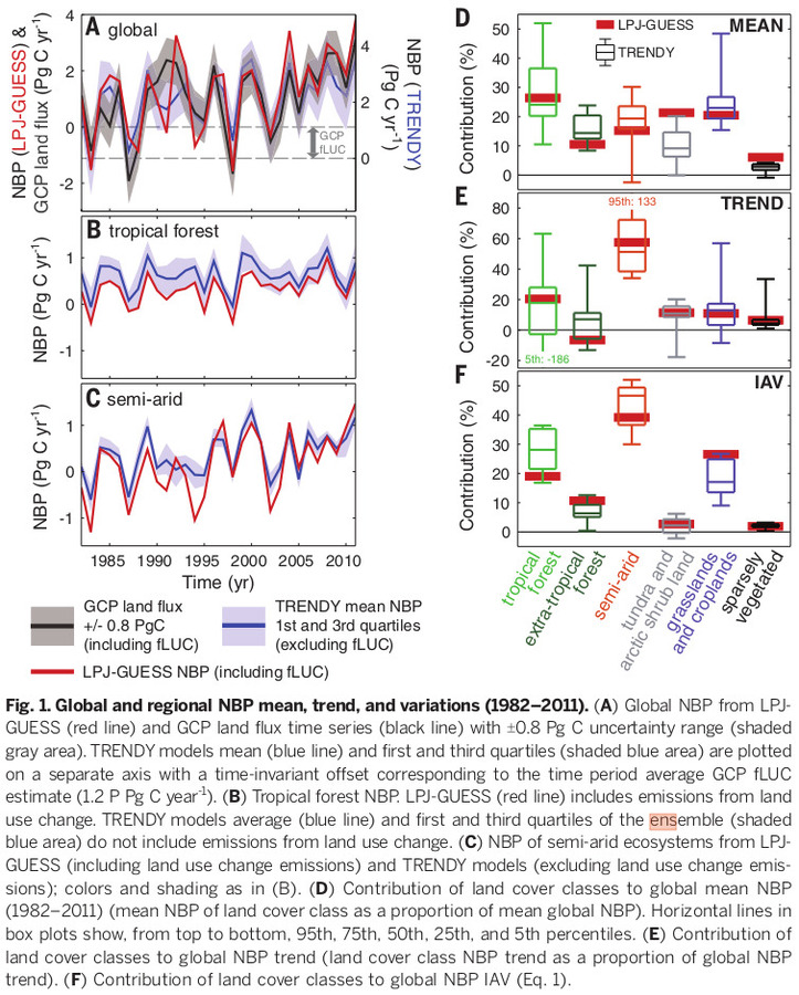
The take-home message was simple and strong. Semi-arid regions dominated the global variability of land carbon sink variability (both long-term trend and interannual variability).

Reasoning: from the bird-eyes-view then zoomed-in view

The reasoning process was also simple and efficient. They compared between LPJ-GUESS and TRENDY ensemble at the global and regional scales. From this, they got the take-home message. Also, they found that GPP, among the carbon cycle components, dominated the regionalvariability.

After the bird-eye-view analysis, they zoomed into the hot spots, trying to see 1) which environmental drivers dominated the variability in semi-arid regions and 2) how this relationship changes with spatial scales.

From this, they found that climatic extreme events (i.e. ENSO) dominated the NBP IAV in semi-arid region. Cool and moist conditions caused positive extreme, while warm and dry ones did the opposite.

With larger spatial scale, precipitation gets more strongly correlated with NBP IAV, implying an important effect of soil moisture on the global NBP IAV.

Quantifying contribution

This paper shares a similarity of methodologies with my current study on TWS. I would call this paper as a carbon cycle version of mine.

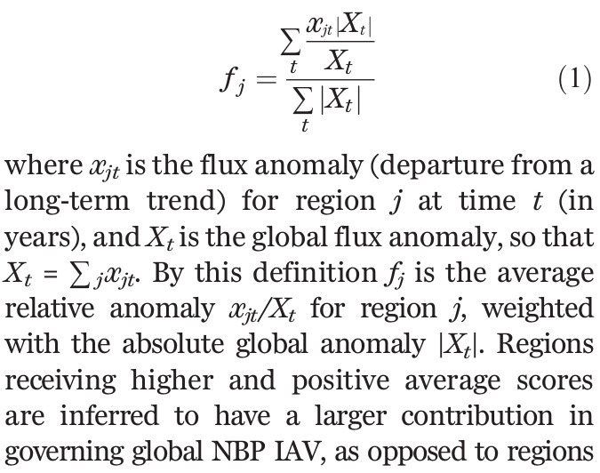
On top of temporal decomposition (i.e. long-term trend and IAV), I would like to mention how they quantified regional contribution to the global NBP IAV.

Accroding to eq. 1, they calculated a contribution factor for each region. Here are some properties of the factor:

• the value is propotional to the contrib. (i.e. large value –> large contrib.)

• the sign of global anomaly value affects the sign of regional contrib.

  • negative anomaly year –> positive anomaly regions contribute negatively to the global IAV
  • positive anomaly year –> positive anomaly regions contribute positively

So, this factor says how each region contributes to result in the globla signal (sign).

This is one of the differences from my method. I am using a way with covariance matrix to quantify regional contributions. The covariance matrix method don’t say the contirubion along with the global signal; it says the original signal of regions. That is, if they have contibuted positively, then they have positive sign regardless of the global signal.

One the other difference is that the covariance matrix way is useful to compare the contrib. among elements. The sum of all elements is 1. So, with the absolute value, one can compare the relative strength as well as the direction via the respective sign.

Anyway, both ways are useful to quantify the contribution of elements to a larger target, as the authors said in supplementary.